Timeseries Classification
This example assumes you’ve read advanced.py, and covers:
- Timeseries binary classification on real data
- Windowed data format; sequence length 188, 4 windows -> 47 points per window
- Binary classification visuals
- Using class weights to handle imbalance
[1]:
import deeptrain
deeptrain.util.misc.append_examples_dir_to_sys_path()  # for `from utils import`

from utils import TS_CONFIGS as C
from utils import init_session, make_timeseries_classifier
from see_rnn import features_1D, rnn_histogram, rnn_heatmap
Dataset info
- PTB Diagnostic ECG Database - https://www.kaggle.com/shayanfazeli/heartbeat
- Number of samples: 14552
- Number of channels: 1
- Number of classes: 2 (binary classification)
- Sampling frequency: 125 Hz
- Datapoints per sequence: 188
Configure TrainGenerator, DataGenerators, & model
[2]:
batch_size = 128
window_size = 188 / 4.  # use 4 windows
assert window_size.is_integer()  # ensure it divides sequence length
window_size = int(window_size)

# Make DataGenerator divide up the (128, 188, 1)-shaped batch
# into 4 slices shaped (128, 47, 1) each, feeding one at a time to model
C['datagen'    ]['preprocessor'] = 'timeseries'
C['val_datagen']['preprocessor'] = 'timeseries'
C['datagen'    ]['preprocessor_configs'] = {'window_size': window_size}
C['val_datagen']['preprocessor_configs'] = {'window_size': window_size}

C['model']['batch_shape'] = (batch_size, window_size, 1)
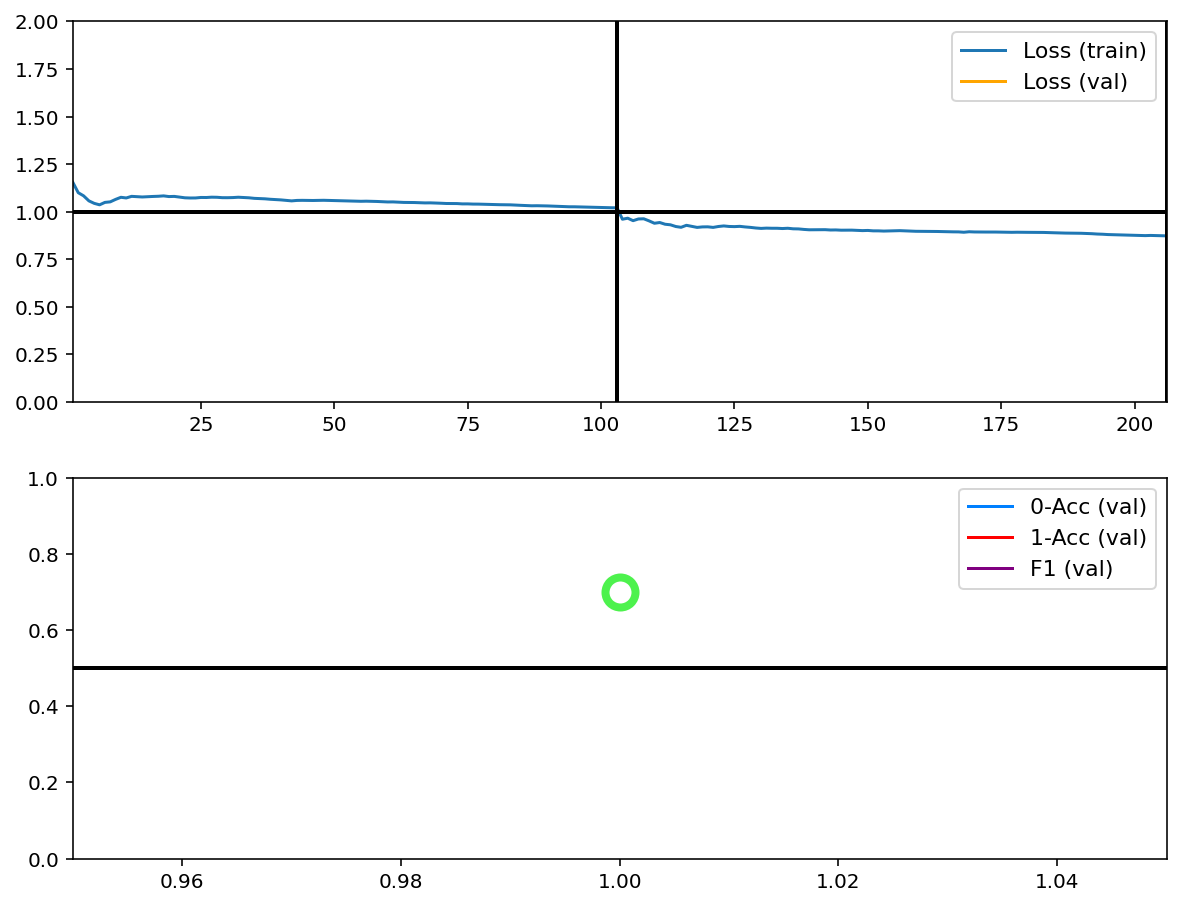
eval_fn: need'predict'for visuals and custom metricskey_metric:'f1_score'for imbalanced binary classificationval_metrics: true positive rate & true negative rate are “class accuracies”, i.e. class-1 acc & class-2 accplot_first_pane_max_vals: plot only validation loss in first plot window, the rest on second, to avoid clutter and keep losses togetherclass_weights: “normal” is the minority class; 3x more “abnormal” samples- others: see utils.py
[3]:
C['traingen'].update(dict(
    eval_fn='predict',
    key_metric='f1_score',
    val_metrics=('loss', 'tnr', 'tpr'),
    plot_first_pane_max_vals=1,
    class_weights={0: 3, 1: 1},
    iter_verbosity=0,
    plot_configs={'fig_kw': {'figsize': (8, 5)},
                  '0': {'legend_kw': {'fontsize': 11}},
                  '1': {'legend_kw': {'fontsize': 11}}},
))
tg = init_session(C, make_timeseries_classifier)
Discovered dataset with matching format
Discovered dataset with matching format
103 set nums inferred; if more are expected, ensure file names contain a common substring w/ a number (e.g. 'train1.npy', 'train2.npy', etc)
DataGenerator initiated

Discovered dataset with matching format
Discovered dataset with matching format
12 set nums inferred; if more are expected, ensure file names contain a common substring w/ a number (e.g. 'train1.npy', 'train2.npy', etc)
DataGenerator initiated

Preloading superbatch ... Discovered dataset with matching format
....................................................................................................... finished, w/ 13184 total samples
Train initial data prepared
Preloading superbatch ... Discovered dataset with matching format
............ finished, w/ 1536 total samples
Val initial data prepared
Logging ON; directory (new): C:\deeptrain\examples\dir\logs\M2__model-adam__max.000
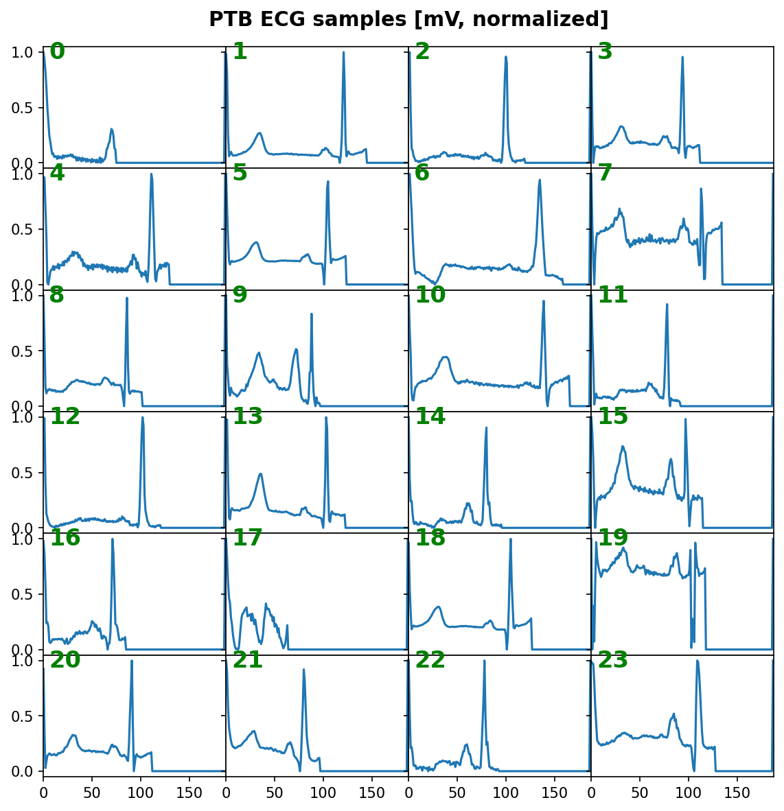
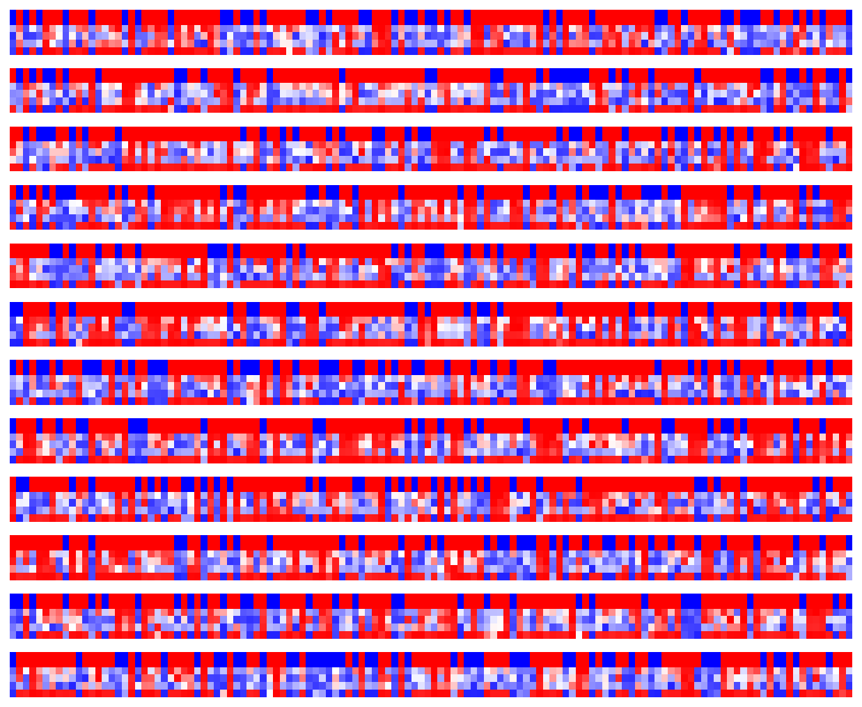
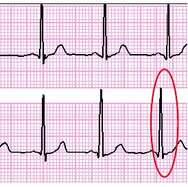
Visualize some samples
[4]:
data = tg.val_datagen.batch
_ = features_1D(data[:24], n_rows=6, subplot_samples=True, tight=True,
                title="PTB ECG samples [mV, normalized]")
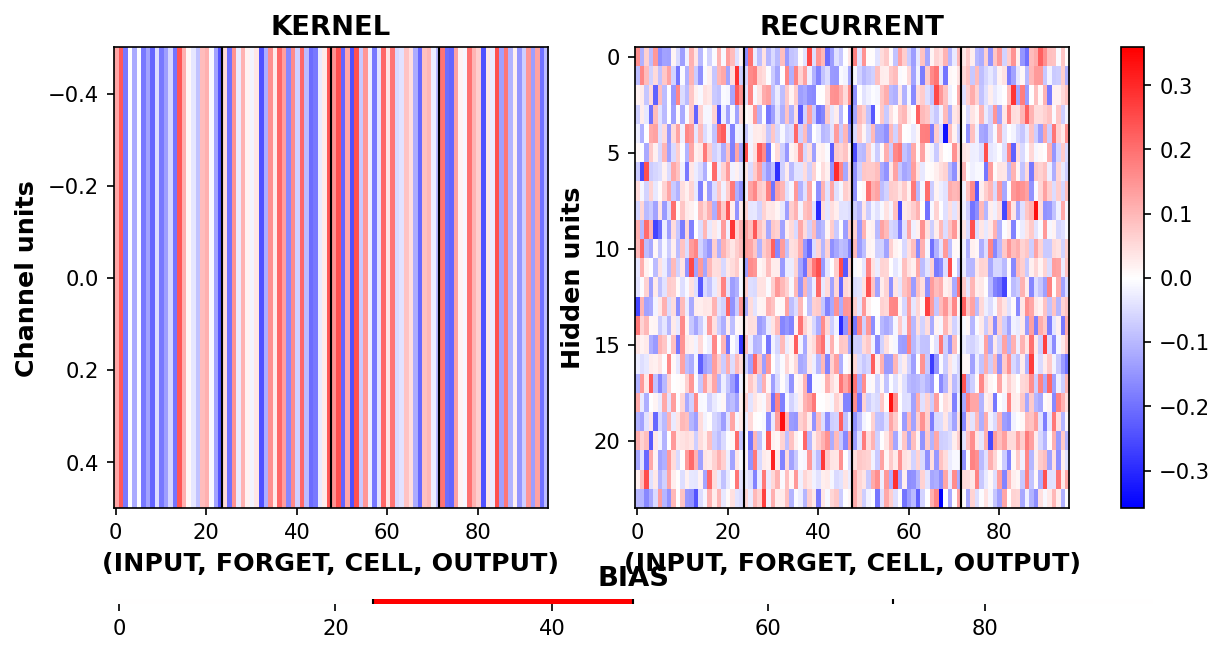
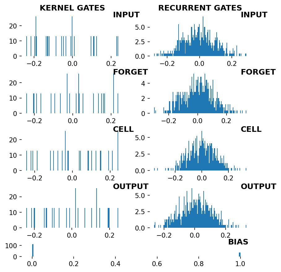
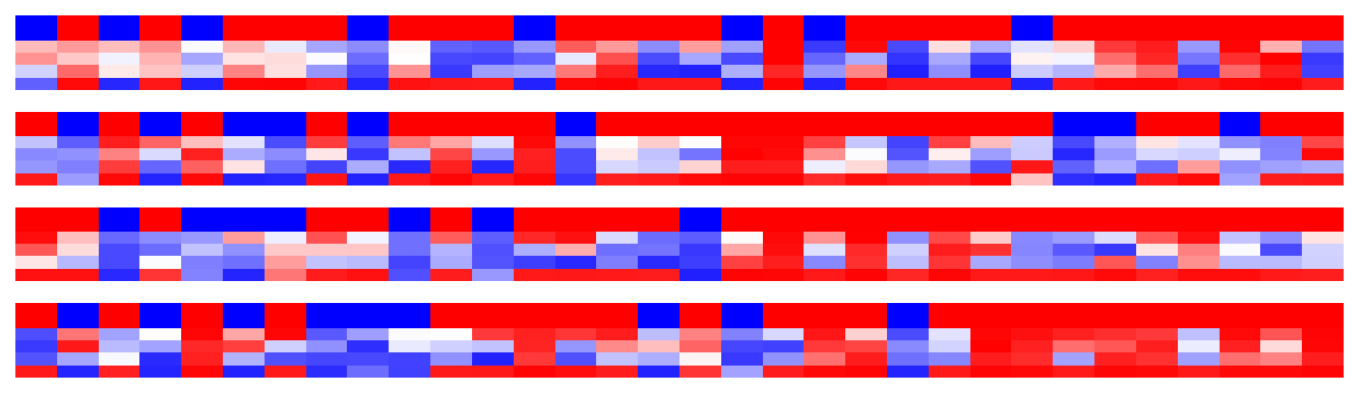
Visualize LSTM weights before training
[5]:
_ = rnn_heatmap(  tg.model, 1, w=.9, h=.9)  # 1 == layer index
_ = rnn_histogram(tg.model, 1, w=.9, h=.9)
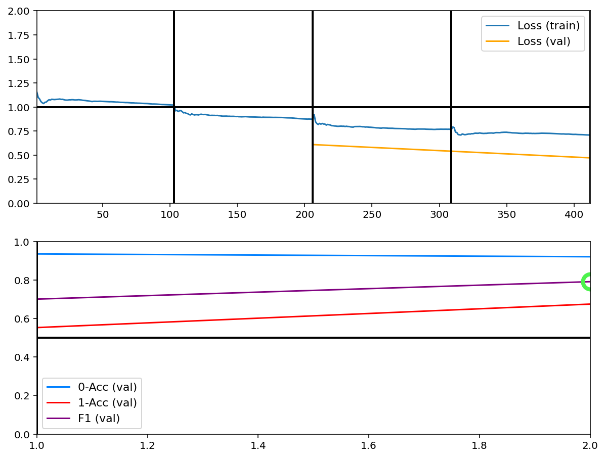
Train
[6]:
tg.train()
Data set_nums shuffled


_____________________
 EPOCH 1 -- COMPLETE


Data set_nums shuffled


_____________________
 EPOCH 2 -- COMPLETE


Validating...
TrainGenerator state saved
C:\deeptrain\deeptrain\visuals.py:577: UserWarning: Attempting to set identical left == right == 1 results in singular transformations; automatically expanding.
  ax.set_xlim(xmin, xmax)
Model report generated and saved
Best model saved to C:\deeptrain\examples\dir\models\M2__model-adam__max.701
TrainGenerator state saved
Model report generated and saved
Data set_nums shuffled


_____________________
 EPOCH 3 -- COMPLETE


Data set_nums shuffled


_____________________
 EPOCH 4 -- COMPLETE


Validating...
TrainGenerator state saved
Model report generated and saved
Best model saved to C:\deeptrain\examples\dir\models\M2__model-adam__max.792
TrainGenerator state saved
Model report generated and saved
Training has concluded.
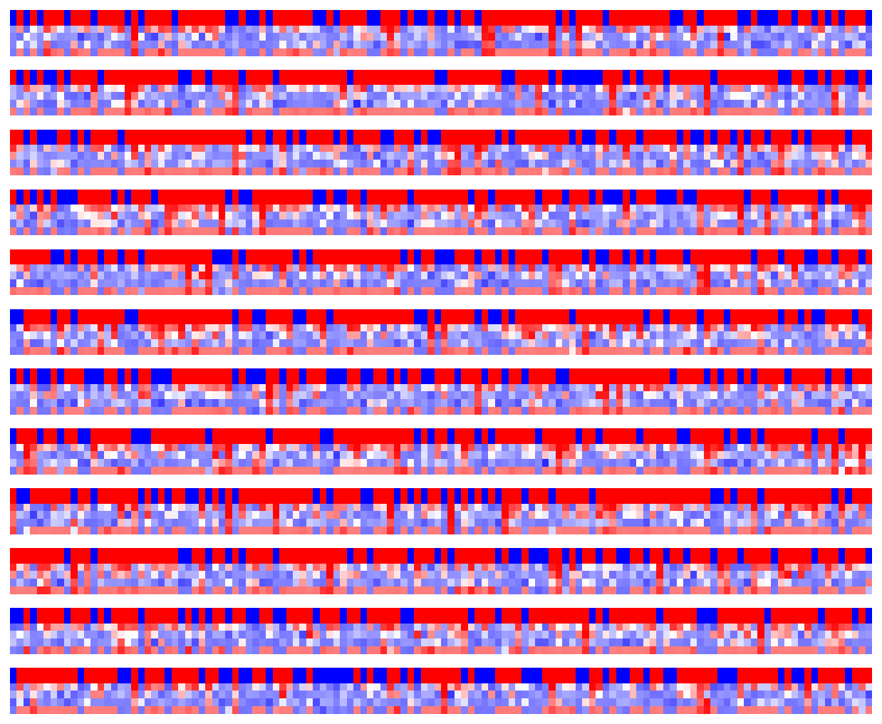
Visualize LSTM weights post-training
[7]:
_ = rnn_heatmap(  tg.model, 1, w=.9, h=.9)  # 1 == layer index
_ = rnn_histogram(tg.model, 1, w=.9, h=.9)
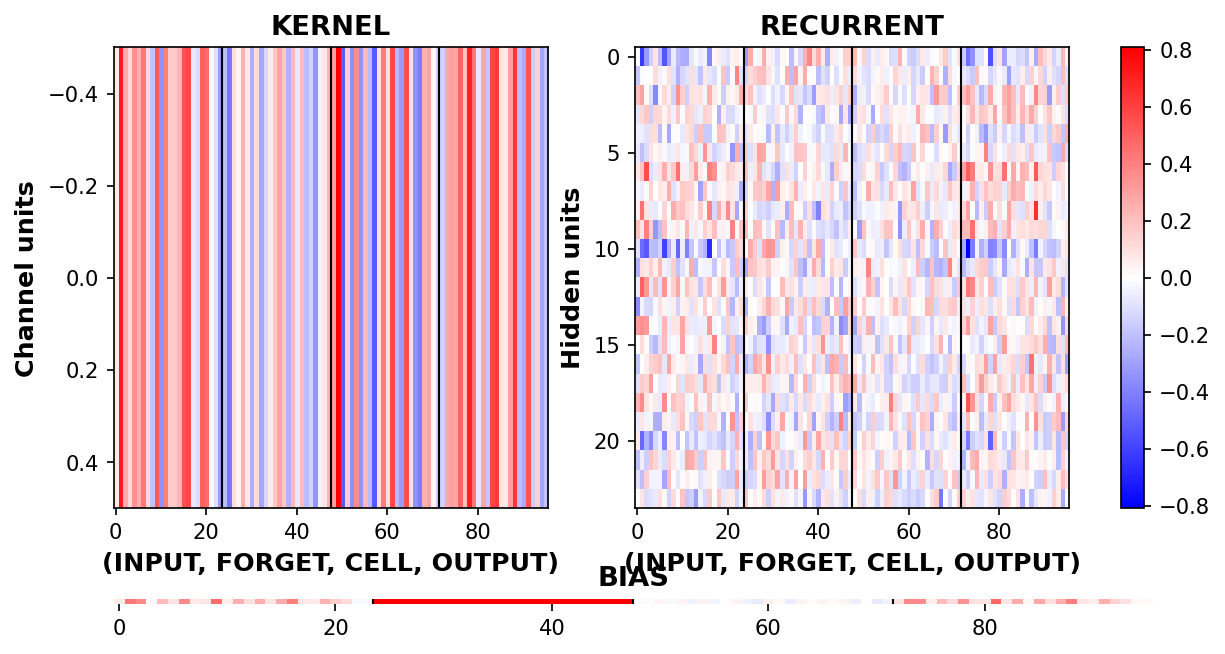
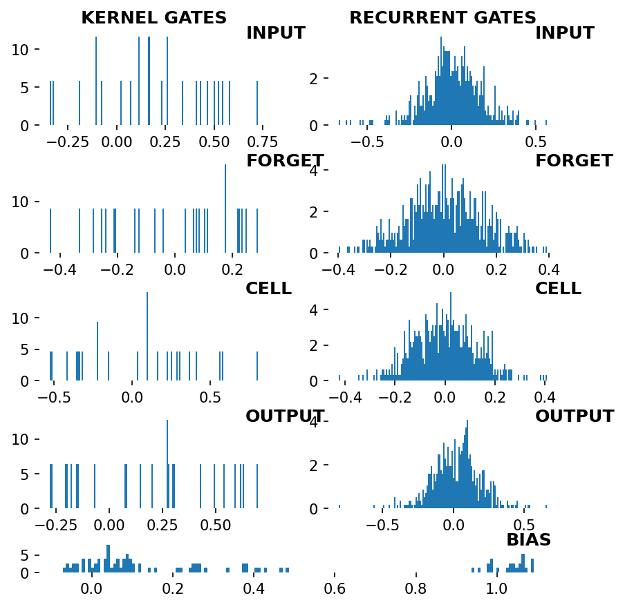
Differences are more pronounced when trained longer.
Next we inspect the callback figures; to redraw them, first we re-validate without clearing cache, to then get predictions & labels from cache for plotting.
[8]:
tg.validate(clear_cache=False, record_progress=False, use_callbacks=False)
Validating...
Predictions per iteration
[9]:
from deeptrain import visuals
import numpy as np
lc = np.asarray(tg._labels_cache)
pc = np.asarray(tg._preds_cache)
# select subset for clearer visual
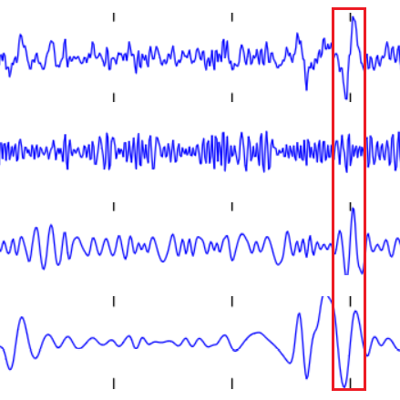
visuals.binary_preds_per_iteration(lc[:4, :, :32], pc[:4, :, :32], h=.9)
- Four “sets” for four batches
- For each set, columns = samples (32)
- Top of each set are labels, plotted with twice the thickness for clarity
- Below the labels are the predictions, heatmapped between blue (0) and red (1)
- Each row of predictions is a timeseries window (“slice”)
Since the model is stateful, if predictions generaly color corretly toward bottom (later windows), it’s indicative of LSTMs utilizing past windows. Here we see no such pattern, but training and tuning were limited.
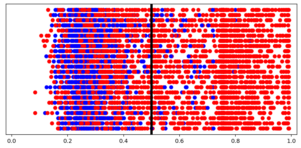
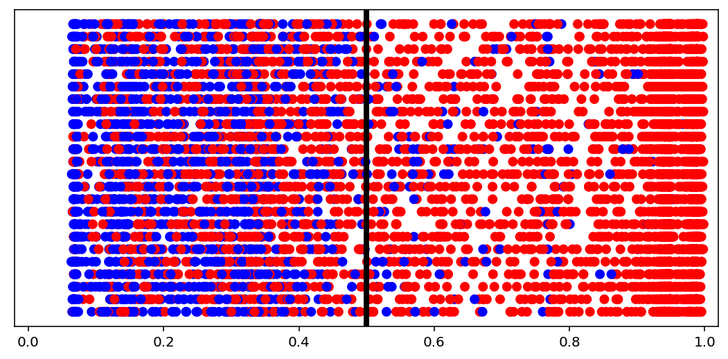
Predictions distribution
[10]:
visuals.binary_preds_distribution(lc, pc, pred_th=tg.predict_threshold)
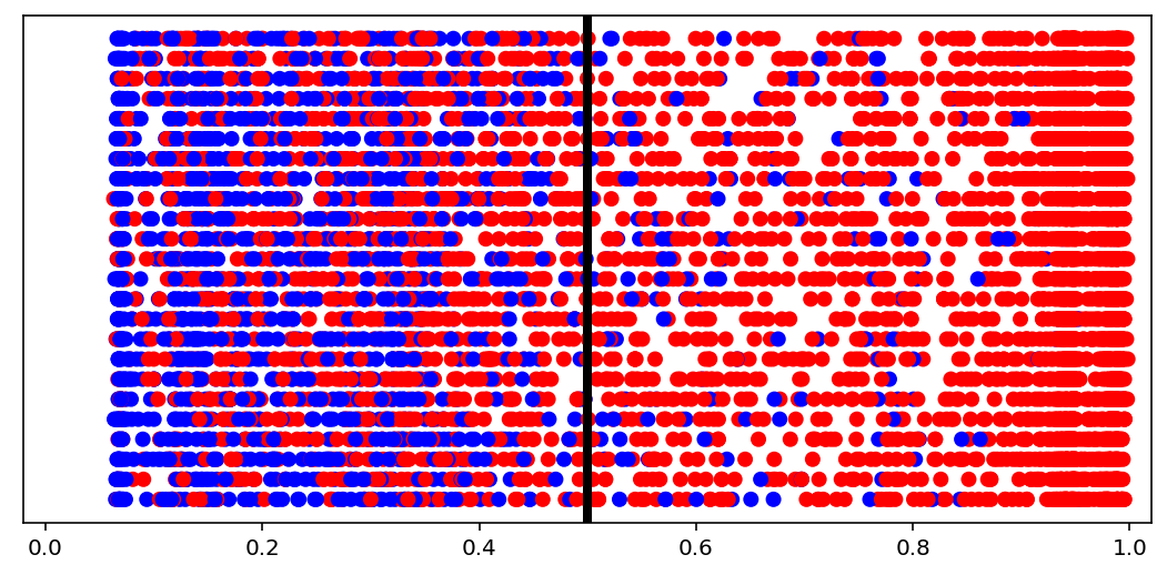
- Dots = predictions
- Red dot at 0.2 = predicted 0.2 for label 1 (red, right of the line = correct)
- Blue dot at 0.2 = predicted 0.2 for label 0 (blue, left of the line = correct)
- Vertical line = prediction threshold
- y-axis is meaningless, vertical space used only to avoid clutter
We see more red dots, as expected (0 is minority), and model being biased toward majority class. A better model will have less red on the left, and less blue on the right. The plot is a good indicator of model “calibration”; sometimes most dots will be either all the way left or all the way right, which may be undesired.
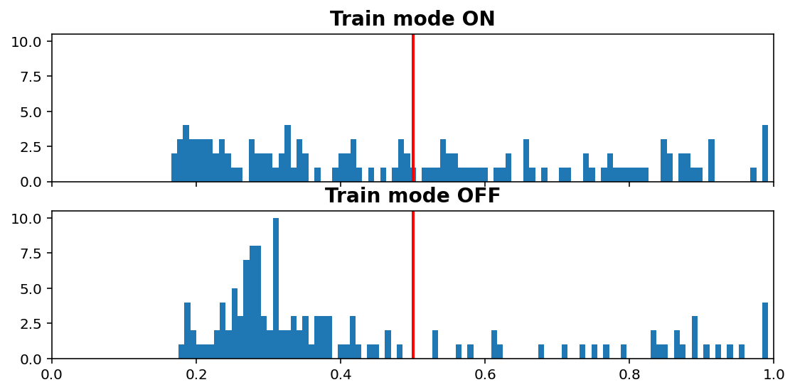
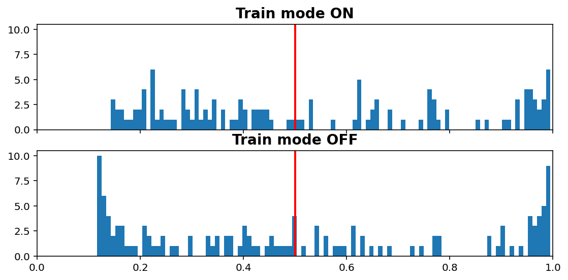
Inference vs. Train histogram
[11]:
visuals.infer_train_hist(tg.model, tg.val_datagen.get(skip_validation=True)[0],
                         vline=tg.predict_threshold, xlims=(0, 1))

- “Train mode” refers to the
learning_phaseflag - When OFF, Dropout rate is 0, Batch Normalization uses moving average instead of batch statistics, and so on
Increasing dropout rate will make ON vs OFF differences more dramatic. Note that the results are only for one validation window; using all would be expensive as we need to compute twice (train & inference), but is doable (see introspection.py).
.........
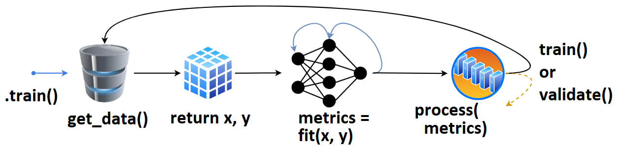
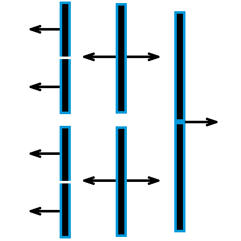
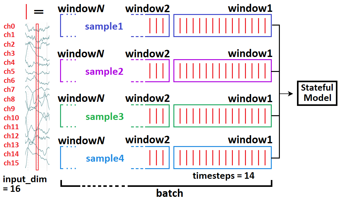
Windowed timeseries idea
- Typical model input shape is
(batch_size, timesteps, input_dim)(below =(4, 14, 16)) - In stateful, we break up a whole batch into “windows”.
- If complete sequence had 70 timesteps, then we’ll feed 5 windows independently (but in right order), then call
model.reset_states() - Relevant: https://stackoverflow.com/a/58277760/10133797
[12]:
from IPython.display import Image
Image(filename='../../docs/source/_images/timeseries_windows.png', width=600)
[12]:
See Preprocessor example on how TimeseriesPreprocessor logic works.